


Next: Discussion
Up: Results
Previous: Influence of the
The relationship between RFs and inhibition schemata can be further
investigated by deriving analytical expressions for their dependence. To
this purpose, to make the problem tractable
we remove the dependence of the kernels on the orientation map, or, in
other terms, we consider an uniform distribution of orientations,
 const
const , e.g.,
  . Under this
assumption,
analytical expressions for the resulting RFs can be easily written, from which
to draw valuable predictions on their properties, and, in general, on the
modus operandi of recurrent inhibition.
Due to the constant orientation map, the structure of the interaction
fields, obtained by the repetition of the same pattern of connections, is
highly regular, so that the effect of recurrent inhibition in the formation
of periodic structures is particularly strong. However, the results should
not to be considered applicable on a narrower scale, compared to those obtained with a
non-constant map. Indeed, a constant distribution of orientation
preferences over the small areas involved in inhibition is just the real
situation within iso-orientation domains, and is a good approximation over
regions with a low orientation drift rate.
Under these conditions, and assuming visual field and cortical plane extending
indefinitely, (9) and (10) can be rewritten as


where  symbolizes the spatial convolution operator and
  denotes both
retinal and cortical coordinates, since the hypothesis of a one-to-one
projection between the visual field and the cortical surface (
 ) still holds.
After convolution theorem, we have

where upper case letters refer to Fourier transforms and  is the
spatial frequency vector.
Rearranging this equation yields

According to our linear setting,  represents the spectral
response profile of the resultant RF and can be readily
calculated from the Fourier transforms of
  and
and  . For the kernels defined by (12) and (16)
and assuming
  ,
,
 is given by

where  and
and  are the components of spatial frequency vector
 .
First, let's infer from (26) a limiting condition on b
to avoid unstable behavior, in relation with the geometrical parameters of the
inhibitory kernel:

Then, we can use this explicit form of  to understand how the
resultant RF depends on the geometrical parameters (
 ,
,  ,
and d) of the kernels and on the strength of inhibition b.
The response properties of a simple cell can be characterized in frequency
domain by comparing the resulting spectrum of its RF with that of a Gabor RF.
To this
purpose, let us consider the frequency tuning curve
  (i.e.,
the frequency sensitivity curve of the simple cell along the axis
orthogonal to the RF orientation), and characterize it by two parameters: the
optimal spatial frequency
  (i.e., the value at which
  gets its peak
value) and the absolute bandwidth
  (i.e., the difference between
the upper (
 ) and lower (
 ) spatial frequencies at which the response amplitude drops to
  of its maximum).
Figure 7 shows a typical dependence of spatial frequency tuning
curves on the parameter b.
An increase of the inhibitory strength b results in a rise of the response
at
  and in a narrowing of the tuning.
For low values of inhibition strength, the spectrum of
  maintain a low-pass structure; for higher values of b two
peaks start growing, symmetrically displaced from the origin. While the center
frequency,
  , of the peaks remains practically constant, the bandwidth,
  , decreases
with b.
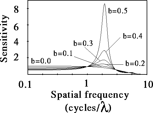
Figure 7:
Frequency tuning curves for increasing values of the inhibition strength
b. Only positive frequencies are shown.
This behavior can be analyzed by considering in detail how inhibition
strength b influences  and
and  , in
dependence on the geometrical parameters of the RF (
 ) and of the
inhibitory kernel (
 and d).
To analyze the effects of the various parameters, it
is convenient to introduce the normalized frequency tuning curve:

where  ,
,  , and
, and  .
.
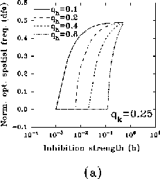
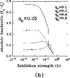
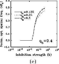
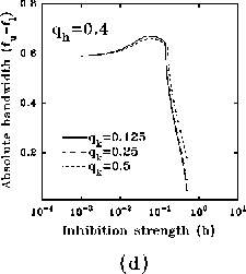
In figure 8a-b, we have plotted, for different values of
 and a typical (fixed) value of
  , the behavior of the normalized
optimal spatial frequency and of the normalized absolute bandwidth versus
the inhibition strength, respectively. Similarly, in
figure 8c-d, the same quantities are represented for
different values of
  and a typical (fixed) value of
  . We observe
a large influence of
  for low values of b, while
increasing the value of b, (i) the normalized optimal spatial
frequency first increases suddenly and afterwards flattens toward an
asymptotic value independent of
  , but dependent on
  , and (ii) the
absolute bandwidth, eventually after a slight increase, quickly drops to a
small fraction of the initial value, independently of
  , and almost of
 .
.
Not a terminal
Figure 8: (click on the image to view a larger version)
Dependence of the normalized optimal spatial frequency (a) and of the
normalized absolute bandwidth (b) for different values of  and
and  .
.
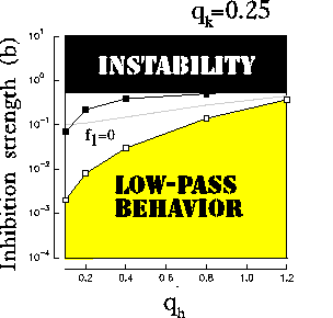
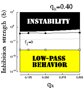
This behavior of  can be summarized in the parameter space as shown
in figure 9a-b (see caption).
 |
 |
| (a) |
(b) |
Figure 9:
(a) Characterization of the resulting RF in the
frequency domain with respect to the parameters b,  , and
, and  .
(a) Influence of variations of the inhibition strength and
of the ratio
  for a fixed value of the ratio
  . The white-square boundary delimits the points for which
  shows a
low-pass behavior (peak-frequency
  ).
The white area contains the points for which a band-pass behavior is
observed, even though, more precisely, only above the grayed line the lower
spatial frequency
  .
The black-square boundary delimits the points for which the
normalized optimal spatial frequency reaches a constant value. Above that
line the normalized optimal spatial frequency practically does not change.
The black-area is the region of system instability, according to
(20). It is worthy to note that for high values of
  we
have a more narrow fractional range of b by which the resulting RF can express
functional diversity.
(b) Similar to (a), but over the parameter plane (b vs.
  ).
We can observe that the parameter of
  is
practically ineffective on the behavior of the resulting RF except for the
slight influence on
  , which defines the boundary of the instability
region (see 20).
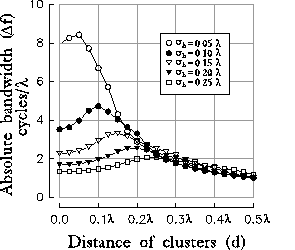
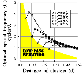
A closer consideration on the specific role of the parameters  and
d is presented in figure 10a-b, where the optimal spatial
frequency and absolute bandwidth are plotted
versus the distance (d) of the clusters for different values of the
initial RF size (
 ) and for a fixed value of the inhibition
strength (
 ).
We can observe that, increasing the distance d, both
 and
and  first rise up and then drop, approaching an asymptotic
value which is independent of
the size
  of the initial excitatory contribution from LGN
projections.
 |
 |
| (a) |
(b) |
Figure 10: (click on the image to view a larger version)
Behavior of the optimal spatial frequency (a) and of the absolute
bandwidth (b) versus the distance of clusters. Different curves correspond
to different sizes of the initial excitatory Gaussian. It is worthy to note
that the frequency tuning curves reach the broadest tuning when the
distance between inhibitory clusters equals the standard deviation
 of the initial contribution from LGN projections.
Let's now consider, how the resulting RF compares with the Gabor RFs in the
spatial domain.
Rearranging (25) yields

where  and
and  are the Fourier transforms of
the equivalent inhibitory kernel in the feed-forward form, and of
the kernel of the over-all open-loop operator, respectively.
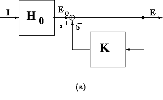
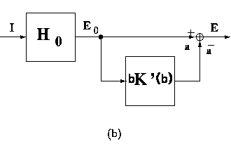
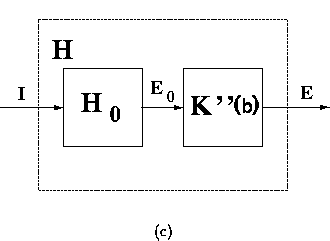
figure 11 illustrates the meaning of these
relations with a block-diagram representation.
Figure 11:
Equivalent block-diagram representations for the recurrent inhibition
schemata. (a) feed-back scheme; (b) equivalent feed-forward inhibitory
scheme; (c) overall transfer function in the open-loop form.
Though the inverse Fourier transform of  is not easy to evaluate, some comments can be evidenced by its Taylor expansion.
If
  , one obtains

Since  is a low pass filter, its powers in (30)
lead to a decrease in bandwidth and so to an increasing width of the coupling
function
[135]. Indeed, back in the space domain the powers of
  result in a sum of
shifted Gaussians with alternating signs, with a considerable increase of the
effective coupling function. Specifically, as the power grows the number of
Gaussians increases as well as their width, while their contribution on the
coupling decreases:

where

The expression for the open loop kernel well evidences the regular distribution
of the additional induced coupling and impacts on the spatial structure of
simple cell RFs.
Specifically, by combining (31) and (32) with
(29), it is easy to obtain a series expression for the resultant
RF after inhibition:

where


We observe that the resulting RF appears as a sum of displaced elongated
Gaussians which
resembles the simple cell models based on differences of offset Gaussians (DOOG)
[52,53,106]. Summing up the Gaussians, for typical values of the parameters
(a sum limited to l=3 is sufficient to have an error
smaller than  for
for  ), we obtain a well-defined Gabor-like
profile, as predicted by DOOG models.
More precisely, the progressive enlarging of the Gaussians with their offset
distance, predicts that the successive sidebands in the resulting RFs are
increasingly widely spaced out, as predicted by the Gaussian derivative model
[128].
From the examination of
the spatial separation of the RF subregions, and by their length
in the direction parallel to the axis of orientation we can make some
considerations on the effects of the model parameters on the orientation
specificity of the resulting RF.
To this end, we have
evaluated from (33) and (34) the aspect ratio
relative to the central subregion,
determined at
  of the peak height, for different initial orientation
biases (p) and for different values of
  . The results, for a
fixed value of the inhibition strength (
 ), are plotted in
figure 12 versus the distance of the inhibitory clusters d.
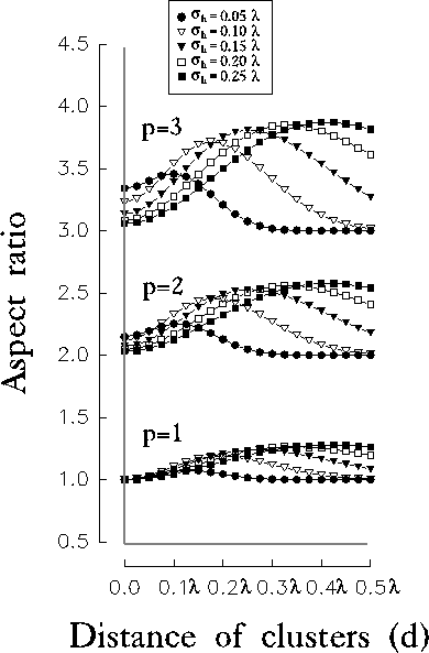
Figure 12:
Aspect ratio relative to the central subregion of the resulting RF,
evaluated at  of its peak value. Each group of curves is related to a
particular value of the initial orientation bias p (i.e., the aspect
ratio of the initial excitatory contribution from LGN).
In all cases, the plots are bell-shaped, evidencing that for each value of
the size of the excitatory contribution  , there exists a value of
d for which we obtain the best improvement in orientation specificity.
Increasing the amount of the initial orientation bias, the effect of
inhibition in improving orientation tuning becomes much more stronger,
anyway, the couples of values
  corresponding to the maxima of
the aspect ratios seem to be independent of the initial orientation bias.
Moreover, it is worthy to note that a slight improvement in orientation can
be observed also without any initial bias (i.e., p=1). Hence, the kind of
intracortical inhibition proposed in our model is able to break circular
symmetries from LGN projections and therefore provides cues for the
intracortical origin of orientation selectivity.


Next: Discussion
Up: Results
Previous: Influence of the
 const
const , e.g.,
  . Under this
assumption,
analytical expressions for the resulting RFs can be easily written, from which
to draw valuable predictions on their properties, and, in general, on the
modus operandi of recurrent inhibition.
Due to the constant orientation map, the structure of the interaction
fields, obtained by the repetition of the same pattern of connections, is
highly regular, so that the effect of recurrent inhibition in the formation
of periodic structures is particularly strong. However, the results should
not to be considered applicable on a narrower scale, compared to those obtained with a
non-constant map. Indeed, a constant distribution of orientation
preferences over the small areas involved in inhibition is just the real
situation within iso-orientation domains, and is a good approximation over
regions with a low orientation drift rate.


 symbolizes the spatial convolution operator and
  denotes both
retinal and cortical coordinates, since the hypothesis of a one-to-one
projection between the visual field and the cortical surface (
 ) still holds.

 is the
spatial frequency vector.
Rearranging this equation yields

 represents the spectral
response profile of the resultant RF and can be readily
calculated from the Fourier transforms of
  and
and  . For the kernels defined by (
 ,
,
 is given by

 and
and  are the components of spatial frequency vector


 to understand how the
resultant RF depends on the geometrical parameters (
 ,
,  ,
and d) of the kernels and on the strength of inhibition b.
The response properties of a simple cell can be characterized in frequency
domain by comparing the resulting spectrum of its RF with that of a Gabor RF.
To this
purpose, let us consider the frequency tuning curve
  (i.e.,
the frequency sensitivity curve of the simple cell along the axis
orthogonal to the RF orientation), and characterize it by two parameters: the
optimal spatial frequency
  (i.e., the value at which
  gets its peak
value) and the absolute bandwidth
  (i.e., the difference between
the upper (
 ) and lower (
 ) spatial frequencies at which the response amplitude drops to
  of its maximum).
Figure
  and in a narrowing of the tuning.
For low values of inhibition strength, the spectrum of
  maintain a low-pass structure; for higher values of b two
peaks start growing, symmetrically displaced from the origin. While the center
frequency,
  , of the peaks remains practically constant, the bandwidth,
  , decreases
with b.

 and
and  , in
dependence on the geometrical parameters of the RF (
 ) and of the
inhibitory kernel (
 and d).
To analyze the effects of the various parameters, it
is convenient to introduce the normalized frequency tuning curve:

 ,
,  , and
, and  .
.
 and a typical (fixed) value of
  , the behavior of the normalized
optimal spatial frequency and of the normalized absolute bandwidth versus
the inhibition strength, respectively. Similarly, in
figure
  and a typical (fixed) value of
  . We observe
a large influence of
  for low values of b, while
increasing the value of b, (i) the normalized optimal spatial
frequency first increases suddenly and afterwards flattens toward an
asymptotic value independent of
  , but dependent on
  , and (ii) the
absolute bandwidth, eventually after a slight increase, quickly drops to a
small fraction of the initial value, independently of
  , and almost of
 .
.
 and
and  .
. can be summarized in the parameter space as shown
in figure

 , and
, and  .
(a) Influence of variations of the inhibition strength and
of the ratio
  for a fixed value of the ratio
  . The white-square boundary delimits the points for which
  shows a
low-pass behavior (peak-frequency
  ).
The white area contains the points for which a band-pass behavior is
observed, even though, more precisely, only above the grayed line the lower
spatial frequency
  .
The black-square boundary delimits the points for which the
normalized optimal spatial frequency reaches a constant value. Above that
line the normalized optimal spatial frequency practically does not change.
The black-area is the region of system instability, according to
(20). It is worthy to note that for high values of
  we
have a more narrow fractional range of b by which the resulting RF can express
functional diversity.
(b) Similar to (a), but over the parameter plane (b vs.
  ).
We can observe that the parameter of
  is
practically ineffective on the behavior of the resulting RF except for the
slight influence on
  , which defines the boundary of the instability
region (see 20).
 and
d is presented in figure
  ) and for a fixed value of the inhibition
strength (
 ).
We can observe that, increasing the distance d, both
 and
and  first rise up and then drop, approaching an asymptotic
value which is independent of
the size
  of the initial excitatory contribution from LGN
projections.


 of the initial contribution from LGN projections.
 and
and  are the Fourier transforms of
the equivalent inhibitory kernel in the feed-forward form, and of
the kernel of the over-all open-loop operator, respectively.
figure
 is not easy to evaluate, some comments can be evidenced by its Taylor expansion.
If
  , one obtains

 is a low pass filter, its powers in (
 result in a sum of
shifted Gaussians with alternating signs, with a considerable increase of the
effective coupling function. Specifically, as the power grows the number of
Gaussians increases as well as their width, while their contribution on the
coupling decreases:


 for
for  ), we obtain a well-defined Gabor-like
profile, as predicted by DOOG models.
More precisely, the progressive enlarging of the Gaussians with their offset
distance, predicts that the successive sidebands in the resulting RFs are
increasingly widely spaced out, as predicted by the Gaussian derivative model
[
 of the peak height, for different initial orientation
biases (p) and for different values of
  . The results, for a
fixed value of the inhibition strength (
 ), are plotted in
figure
 of its peak value. Each group of curves is related to a
particular value of the initial orientation bias p (i.e., the aspect
ratio of the initial excitatory contribution from LGN).
 , there exists a value of
d for which we obtain the best improvement in orientation specificity.
Increasing the amount of the initial orientation bias, the effect of
inhibition in improving orientation tuning becomes much more stronger,
anyway, the couples of values
  corresponding to the maxima of
the aspect ratios seem to be independent of the initial orientation bias.
Moreover, it is worthy to note that a slight improvement in orientation can
be observed also without any initial bias (i.e., p=1). Hence, the kind of
intracortical inhibition proposed in our model is able to break circular
symmetries from LGN projections and therefore provides cues for the
intracortical origin of orientation selectivity.