
As the building block, the model of a single oscillator is defined in the simplest form as a feedback loop between an excitatory unit and an inhibitory unit (Figure 1a):
where  and
and  are positive parameters describing the coupling
between the two units. Adding an
inhibitory feedback to the inhibitory unit as in
[63,71] does not seem to
change the qualitative behavior.
  represents the input from other
oscillators and
  represents external stimulation.
  is a
decay parameter, and
  denotes the amplitude of a Gaussian noise term.
 is a sigmoid gain function with threshold
  ,
where
  , and parameter T.
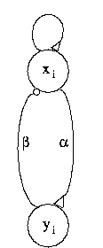 |
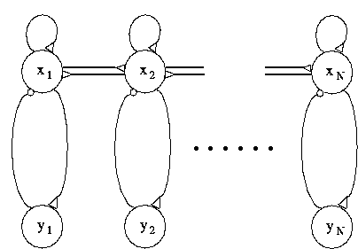 |
| |
|
 and an inhibitory unit
 .
.  and
and  are mutual connection strengths. ( b)
A chain of N oscillators. Small triangles indicate excitatory connections,
and small circles inhibitory connections.
Equation 2 is essentially a simplification of the Wilson and Cowan oscillators
[72], and it has been shown that the system produces
oscillations within a wide range of parameters
[3,72]. Figure 2 shows a typical limit cycle drawn on the x-y plane,
as exhibited by a single oscillator. The two nullclines split the x-y
plane
into four regions. Within each region,  and
and  have unique signs.
For example,
  and
and  in the upper-left region (where the
starting point lies in). Thus, both x and y decrease in this region until
the trajectory intersects with the x-nullcline. After the intersection, the
trajectory moves into the lower-left region where
  and thus x
starts to increase. Following this type of qualitative analysis, one can
see why (2) gives rise to oscillations. As in the following simulations,
the equations were numerically solved with the simple Euler method, where
 . The results were also confirmed using the fourth-order
Runge-Kutta method. The oscillator model can be biologically interpreted
as a mean field approximation to a network of excitatory and inhibitory
neurons
[7,23,56].
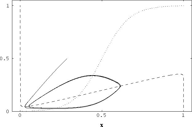
Figure 2: Nullclines and limit cycle trajectory of
a single oscillator as shown in the phase plane. The x-nullcline
( ) is shown by the dashed curve and the y-nullcline (
 )
is shown by the dotted curve. The oscillator started from a randomly
generated point, the end point near (0.3, 0.5), and it quickly fell
in the trajectory of a limit cycle. The parameters for this simulation
are
  = 0.3,
  = 2.5,
  = 0.01,
  = 0.2,
 = 0.15, T = 0.025,
  = 1.0, and I = 0.2.
2,000 integration steps.
To see the detailed behavior of an isolated oscillator, Figure 3 presents the
simulation of the system with different parameters. Figure 3a shows that if
the external input is very small, the oscillator will be silent; but if the
input is very high the system reaches a saturation point. Oscillations
(limit cycles) occur between the two extremes. In other words, oscillations
are driven by input, as opposed to the phase model where oscillation is built
into the system. Figure 3b shows that  controls the frequency of oscillations, and Figure 3c demonstrates that
 has a major influence on the amplitude of oscillations.
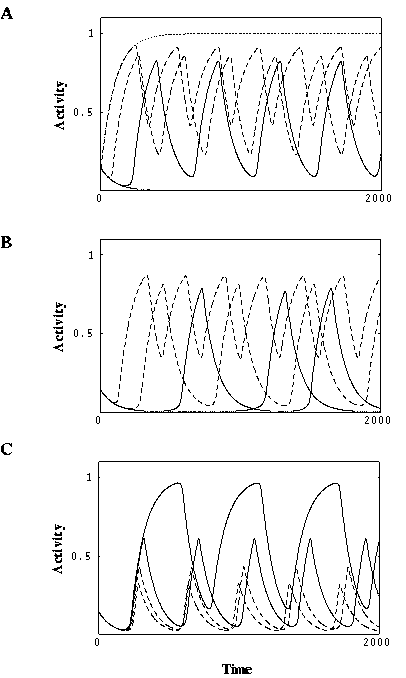
Figure 3: Behavior of a single oscillator.
( a) Effect of varying external input. Solid thick, I = 0.0;
solid thin, I = 0.2; dashed thick, I = 0.4; dashed thin, I = 0.8;
dotted, I = 1.6.  = 1.0 and
  = 0.2. ( b)
Effect of varying
  . Solid thick,
  = 0.2; solid thin,
 = 0.4; dashed thick,
  = 0.8; dashed thin,
  = 1.6.
 and
and  = 0.2. ( c) Effect of varying
  .
Solid thick,
  = 0.15; solid thin,
  = 0.3; dashed thick,
 = 0.45; dashed thin,
  = 0.6.
  and
and  = 1.0.
The other parameters are the same as in Figure 2. 2,000 integration steps.
Weak coupling between oscillators ( is relatively small) does not disrupt
the oscillatory behaviors of individual oscillators. To study the properties
of a network of oscillators, first a chain of N oscillators is constructed
with only neighboring coupling between excitatory units, as shown in Figure 1b.
We define the coupling as
where W is a connection weight. Note that the weights of the connections to
the two end oscillators 1 and N double those of the connections to the other
interior ones in the chain. We found, with uniform external input and
random values for  and
and  (namely random phases) initially, that the
chain with coupling (3) is synchronized after an initial period of rapid phase
transitions. The synchronization is absent, however, if the connections
to the end oscillators are equally strong as to the interior ones.
Instead we found phase shifts across the chain. Figure 4presents a
simulation with N = 30. Note that there were small phase differences when
nearly stable limit cycles started to occur, but the differences diminished
as time went on.
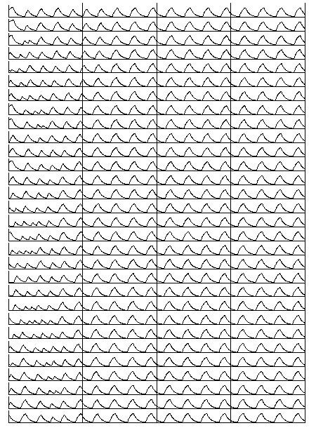
Figure 4: Synchrony in a chain of oscillators.
The input  , and the initial values
  and
and
 were randomly generated within the range
[ 0.8,0]. The height
of the ordinate of each oscillator is 1.
  and N = 30.
The parameters
  ,
,  , and the remaining ones are
the same as in Figure 2. 8,000 integration steps. Vertical lines are
drawn to help identify phase relations among the oscillators.
A chain of oscillators using the phase model has been extensively studied for modeling swimming behaviors in fish [11,33]. Cohen et al. [11] noted that phase-locking with no phase shift can be reached with a chain of identical oscillators. However, phase-locking cannot be produced if there is inhomogeneous input to a chain, contradicting the experimental conditions of Gray et al [24], where synchrony can occur even if two stimulus bars are not connected (more discussion in the Modeling Cortical ... section). For this reason, the chain model was considered not proper for modeling the phase locking experiments [30]. But, as will be clear later, our model does not suffer from this problem.
(3) is not a necessary condition for phase-locking. Let us call an
oscillator active if it receives an external stimulus. We observed that in
a system defined by (3), as long as the overall (sum of) weights of the
connections converging on every active oscillator from all other active
oscillators are kept constant, phase-locking occurs. This condition is
called the equal weight condition. (3) is a special
case of this condition.
It is easy to show that without noise ( ) homogeneous input
leads to the
solution of synchronized oscillations to (2). When the system is in
synchrony,
  , for
, for  . With the equal weight
condition, we have
  , and thus
  , and
, and
 , for
, for  . Therefore, the system will keep the synchrony in its
evolution. The stability of the synchronized solution remains to be
analyzed. Extensive numerical simulations have been conducted, however,
and we found that the system is stable with respect to perturbations by
noise once it reaches synchronous
oscillations
 .
Intuitively, positive
coupling between neighboring oscillators serves to drive the oscillators
close to each other in phase and it can also correct small discrepancies
among the phases of the oscillators. We have tested one dimensional
chains of up to 256 oscillators and two dimensional grids of up to 100 by
100, and synchrony in such systems is stable. So even the conclusion
concerning long range synchrony might not be established when the size
of the network tends to infinity, the significance of the system studied
here does not vanish because almost all practical applications of
oscillator networks, such as image analysis (see the Why Local ... section), require
only limited sizes.
The equal weight condition is easily achieved if one allows connection
weights to be dynamically modified on a fast time scale, an idea first
introduced by von der Malsburg
[62]. In this scheme, there is a pair
of connection weights from oscillator j to i, one permanent  , and
another dynamic
  (so called Malsburg synapses, see
[12]).
Permanent links reflect the hardwired structure of a network, while dynamic
links quickly change from time to time. In computations, though, only
dynamic links formed on the basis of permanent links play an effective role.
The equal weight condition can be naturally realized by a modification rule
of dynamic links which combines a Hebbian rule
[27] that
emphasizes coactivation of oscillators i and j and a normalization of
all incoming connections to an oscillator. More specifically, it can be
implemented by a two-step procedure: First update dynamic links and then
normalization:
where  and
and  are positive parameters, and function
  measures whether x is active. It is here simply defined as
  if <x> is greater than a constant and
  otherwise,
where the angular bracket <x> stands for temporal averaging of the
activity x.
 is introduced to
prevent division by zero. Note that weight normalization of this form
is commonly used in neural network models for competitive learning
[22,61].
With introduction of fast changing synapses, the equal weight condition in
(3) can now be
reached by dynamics in (4) from a natural condition  , and
, and  defined for
permanent links, where T
is the strength of every permanent link. In other words, the same
permanent link is established for only neighboring oscillators, and there
is no permanent connection beyond nearest neighbors. Because of this,
dynamic links can be established for only neighboring oscillators
according to (4a). Since the entire chain is stimulated,
  for
for
 . Following (4), after a very brief beginning period,
 if oscillators i and j are nearest neighbors and
 1 or N. Additionally,
  . This
connection pattern of dynamic (effective) links is equivalent to (3) if
one lets
  .
.
It should be obvious that the result concerning global synchrony extends to oscillator networks of higher dimensions than 1-D. A prototype of 2-D network is illustrated in the Modeling Cortical ... section. Also, the result is established for lateral connections beyond nearest neighbors. Indeed, more extensive connections can speed up the synchronization process. In a sense, synchrony in fully connected networks is a special case of our result based on local coupling.