next up previous contents
Next: 5.6 Conclusion Up: 5 Aftereffect Experiments Previous: 5.4 Changes in the

5.5 Time course of the tilt aftereffect

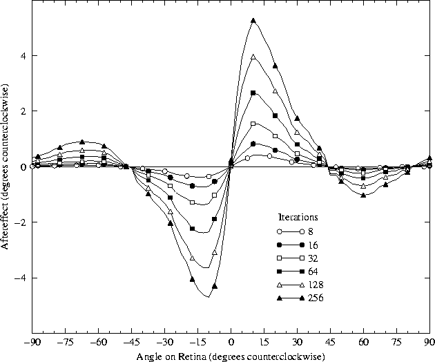
  In addition to the angular changes in the TAE described in the previous sections, the magnitude of the TAE in humans increases regularly with adaptation time (Gibson and Radner, 1937). The equivalent of ``time'' in the RF-LISSOM model is an iteration, i.e. a single cycle of input presentation, activity propagation, settling, and weight modification. Figure 5.9 shows how the TAE varies for each angle as the number of adaptation iterations is increased.
 
Figure 5.9: Tilt aftereffect versus angle over the course of adaptation.
  Each curve shows the average TAE in the RF-LISSOM model from figure 5.2 with a different amount of adaptation. The same basic S-shaped curve is seen regardless of the duration of adaptation, but the magnitude increases monotonically with adaptation.
\begin{figure}
\centering
 \hputpictype{\psline} 970101_ae_090d_avg.neg.setl (\xmgrplotwidth) 
 \end{figure}

The same basic S-shaped curve is always evident, but its magnitude increases monotonically with adaptation. Since obtaining human data for even a single curve is extremely time consuming, equivalently comprehensive data for human subjects is unavailable. The plots are easily obtained for the model, however, which illustrates one reason why computational models are important -- they make it possible to obtain quite detailed data that can constitute predictions for later experimental work.

The experimental work that has been done so far on the time course of the TAE in humans (Gibson and Radner, 1937; Greenlee and Magnussen, 1987; Magnussen and Johnsen, 1986) corresponds to a single vertical slice through the direct TAE region in figure 5.9. It is measured by presenting an oriented adaptation figure for an extended period interrupted at intervals by the presentation of test and comparison lines. At each test presentation, the amount of the TAE present is measured using the standard techniques illustrated in figure 2.3. The duration of the test presentation is minimized so that it will not affect the magnitude of the TAE significantly.

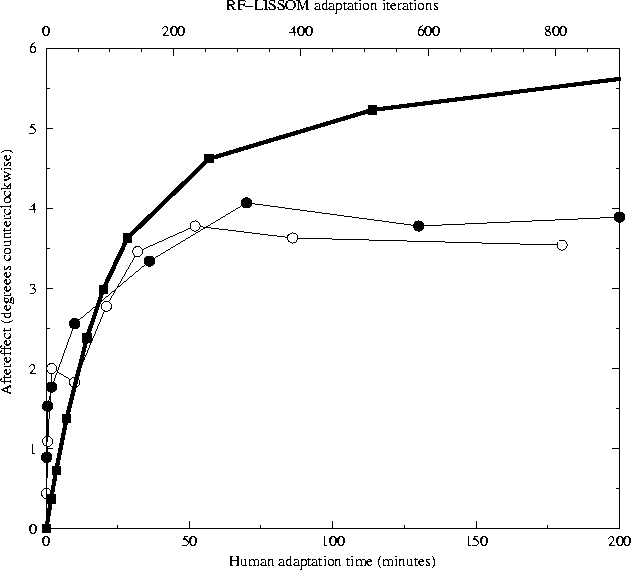
When the time course of the direct TAE is measured in this way for human subjects, the increase is approximately logarithmic with time (Gibson and Radner, 1937), as is evident for the model in figure 5.9. The magnitude of the TAE eventually reaches saturation at a level that depends upon the experimental protocol used (Greenlee and Magnussen, 1987; Magnussen and Johnsen, 1986). Figure 5.10 compares the shape of the TAE versus time curve for human subjects and for the RF-LISSOM model.

 
Figure 5.10: Direct tilt aftereffect versus time.
  The circles show the magnitude of the TAE as a function of adaptation time for human subjects MWG (unfilled circles) and SM (filled circles) from Greenlee and Magnussen (1987); they were the only subjects tested in the study. Each subject adapted to a single +12° line for the time period indicated on the horizontal axis (bottom). To estimate the magnitude of the aftereffect at each point, a vertical test line was presented at the same location and the subject was requested to set it a comparison line at another location to match it. The vertical location of each point represents the average of five settings; the data for 0 - 10 minutes were collected separately from the rest. For comparison, the heavy line shows average TAE in the LISSOM model for a +12° test line over 9 trials (with parameters as in figure 5.2). The horizontal axis (top) represents the number of iterations of adaptation, and the vertical axis represents the magnitude of the TAE at this time step. The RF-LISSOM results show a similar logarithmic increase in TAE magnitude with time, but do not show the saturation that is seen for the human subjects.
\begin{figure}
\centering
 \hputpictype{\psline} 970101_ae_090d_avg.setl_wrt_time.compared_to_GM87 (\xmgrplotwidth) 
 \end{figure}

The x axis for the RF-LISSOM and human data has different units, but the correspondence between the two curves might provide a rough way of quantifying the equivalent real time for an ``iteration'' of the model. The time course of the TAE in the RF-LISSOM model is similar to the human data, but the model does not show saturation effects over the adaptation amounts tested so far. This difference indicates that the biological implementation has additional constraints on the amount of learning that can be achieved over the time scale over which the tilt aftereffect is seen. This issue is explored further in the discussion in the next chapter, including possible ways that saturation might be incorporated into the RF-LISSOM model.


next up previous contents
Next: 5.6 Conclusion Up: 5 Aftereffect Experiments Previous: 5.4 Changes in the
James A. Bednar
9/19/1997