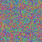
| Demo 5.9. Self-organization of the OR map.
This animation of Figure 5.9 shows
how the LISSOM OR map self-organizes over time. The OR preference, OR
selectivity, and combined preference and selectivity of each neuron in
the LISSOM OR map are shown over 10,000 input presentations (oriented
Gaussian patterns). The OR preference is color coded according to the
key on top, and selectivity represented in gray scale from black to
white (low to high), as in the macaque OR map of Figure 2.4.
(a) The orientation preferences were initially random, but over
self-organization, the network developed a smoothly varying
orientation map. The map contains all the features found in animal
maps, such as linear zones, pairs of pinwheels, saddle points, and
fractures (outlined in Figure 5.9).
(b) Before self-organization, the neurons are unselective (i.e. dark),
but nearly all of the self-organized neurons are highly selective
(light). (c) Overlaying the orientation and selectivity plots (by
representing selectivity with color saturation i.e. its fullness or
intensity) shows that regions of low selectivity in the self-organized
map tend to occur near pinwheel centers and along fractures. (d)
Histograms of the number of neurons preferring each orientation (OR H)
are essentially flat because the initial weight patterns were random,
the training inputs included all orientations equally, and LISSOM does
not have artifacts that would bias its preferences. These plots show
that LISSOM can develop biologically realistic orientation maps
through self-organization based on abstract input patterns.
Next demo
|