Demos: Computational Maps in the Visual Cortex

#!/lusr/bin/php Demos: Computational Maps in the Visual Cortex

Computational Maps in the Visual Cortex
Demo 13.6
Miikkulainen • Bednar • Choe • Sirosh

Home

About the Authors

Back Cover

Table of Contents

Sample Chapter

Figures

References

Errata

Demos

Talks/Courses

Software

Credits

Purchase online at:

0^o
30^o
50^o
70^o


Play/Pause	Reset Animation	Step through	Speed Control

Depending on your connection speed, the animation may take a while to load; it is ready when images appear in the boxes above. The [<] and [>] buttons wrap around; [<] can be used to get to the final frame quickly. Original JavaScript animation source from webreference.com.

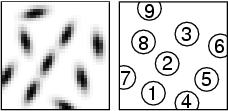
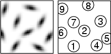
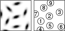
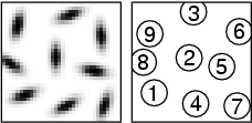
Demo 13.6. Contour integration process. This animated version of Figure 13.6 shows how the neurons in the PGLISSOM orientation map synchronize their spiking activity to represent continuous contours. The input presented to the network is shown in gray-scale coding at left, the areas of the map that respond to the different input elements are delineated with circles in the middle, and the neural spiking in the 54 × 54 GMAP is shown as black and white dots at right (black means the neuron is spiking at the current time step, white means that it is not spiking). Each contour was composed of three contour elements (numbered 1, 2, and 3), embedded in a background of six randomly oriented elements. Each contour runs diagonally from lower left to top right with varying degrees of orientation jitter.

PGLISSOM performs contour integration through synchronized and desynchronized neural activation: Neurons that represent elements of the same contour spike at the same time, and those that represent elements in different contours spike at different times. Through self-organization, principles of good continuation and proximity have become encoded in the excitatory lateral connections, i.e. neurons that represent collinear or co-circular paths tend to be connected. The lateral connections mediate synchronization, and as a result, PGLISSOM groups collinear and co-circular elements together into continuous contours.

This experiment demonstrates contour integration performance with four different degrees of orientation jitter, i.e. misalignment of the contour elements. In all cases, the background elements are unsynchronized. The contour is very strongly synchronized for 0^o and 30^o but relatively weakly synchronized for 50^o and 70^o of orientation jitter. In other words, the contours get harder to detect as the jitter increases, as they do in humans (Figure 13.7). The model therefore gives a computational explanation for the human contour integration process in terms of self-organized lateral connections and synchronization.

Previous demo; Next demo