 |
 |
 |
 |
| 54 x 54 | 72 x 72 | 96 x 96 | 144 x 144 |
| 0.41 hours | 0.77 hours | 1.73 hours | 5.13 hours |
| 8MB | 22MB | 65MB | 317MB |
Self-organizing computational models like RF-LISSOM that have specific intracortical connections can explain many functional features of visual cortex, such as orientation and ocular dominance maps. (If you aren't familiar with orientation maps, first check out our short demo.)
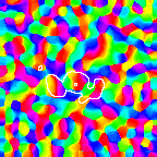
Unfortunately, these models are difficult to simulate because they require large amounts of computer memory to hold the connections, and because they take a lot of computation time. To make the study of larger-scale phenomena practical, we have derived a set of scaling equations that allows small networks to be used as approximations for larger ones, while allowing the same parameters to be used for full-scale simulations once the concept has been demonstrated. For example, here are orientation maps from a wide range of network sizes whose parameters were computed with the scaling equations:
 |
 |
 |
 |
| 54 x 54 | 72 x 72 | 96 x 96 | 144 x 144 |
| 0.41 hours | 0.77 hours | 1.73 hours | 5.13 hours |
| 8MB | 22MB | 65MB | 317MB |
Here the lateral inhibitory weights of one neuron in each map are outlined in white. Even though the initial weights differ in all of these simulations (both in number and value), for a large enough size the results are similar. To see the match, compare each of the corresponding colored blobs between the 96 x 96 and 144 x 144 simulations. For the smallest simulations, precisely matching parameters are not possible due to the discrete values allowed in the small grid. The larger simulations allow a better match, and develop nearly identical maps when presented with the same stream of inputs during training. Thus the RF-LISSOM model predicts that the map patterns seen in animal V1 are primarily due to the input patterns seen by the developing cortex, and not to their initial weights or even many of the details of their architecture. Much larger maps also perform similarly, but are only possible on supercomputers.
With the scaling equations, we can use relatively small simulations for most purposes, and scale up only when necessary to see a certain phenomena. The scaling equations are also of interest for biology, since they facilitate the comparison of biological maps and parameters between individuals and species with different brain region sizes. More details are available in the GLISSOM tech report or in the (shorter) CNS*01 paper.
Even with the scaling equations, simulating scaled-up networks is still difficult because the larger networks take much more simulation time and memory. We are exploring one possible solution, which is to use the scaling equations to dramatically reduce memory and computational requirements by scaling a small network into a larger one during training.
Here's an example of an RF-LISSOM orientation map simulation (on the left) along with a corresponding GLISSOM simulation (on the right):

(Click on the image to launch an MPEG video viewer; the video is 3MB in size and 60 seconds long.) Each frame of this video shows an orientation map from each algorithm at one iteration. At first every other iteration is shown; by the end only every 20th iteration is shown. The GLISSOM map starts out coarse (with fewer, larger pixels than RF-LISSOM), but it is gradually scaled up to match the size of RF-LISSOM. The result is a similar map whose simulation takes only 15MB (compared to RF-LISSOM's 65MB) and 0.65 hours (compared to RF-LISSOM's 1.7 hours):

Importantly, larger networks show greater speedup and memory differences (e.g. 3X and 5X for a 144 x 144 simulation), while larger starting sizes can be used to approach almost arbitrarily close to the RF-LISSOM result in less time and memory.
Calculations suggest that with GLISSOM it should be possible to simulate all of human V1 at the single-column level using existing supercomputers, making detailed study of large-scale phenomena practical. See the GLISSOM tech report for those calculations and for the GLISSOM algorithm and its full speedup and memory savings results.